Basic Data Structure and Algorithm
The sort() function has asymptotic time complexity of O(N*log N)
Why does accessing an Array element take O(1) time?
Array store value in a contiguous manner and array itself is pointer which points to the starting
By adding the product of the index number (of value to be fetched) and the size of one element (ex. int size is 4 bytes) with the base address, we can have the address of that index’s value. we don’t have to iterate through the array. So it’s done in O(1).
In array A[] = {8, 6, 7, 13, 8, 19}
To fetch the value at index 4, we need the memory address where the value of that index is stored. The address can be obtained by doing an arithmetic operation i.e.
Address of value at index 4 = Address of index 0’s value + 4 × size of int = 108 + 4 × 4 bytes Address of value at index 4 = 124 A[4] = value at address 124 = 8
Difference Between Array and Linked List
Definition
An array is a grouping of data elements or data items stored in contiguous memory.
A linked list data structure in which each element is allocated dynamically, and each element points to the next element
Memory Allocation
It stores the data elements in a contiguous memory zone.
It stores elements randomly, or we can say anywhere in the memory zone.
Dependency
The elements are not dependent on each other.
The data elements are dependent on each other.
Size
Fixed
Dynamic
Memory is allocated during
Compile-Time
Run-Time
Access Time
O(1): For direct access using indexes
O(n), since elements need to be traversed sequentially.
Insertion + Deletion
O(n): worst case (when insertion or deletion is done at the beginning or in the middle)
O(1): if insertion is done at the beginning.
O(n): If insertion is done at the end without a tail pointer.
Search Time
O(n): Worst Case (linear search)
O(logN): With binary search if sorted.
O(n): Worst Case (linear search)
Use-Case
When the size is known and fixed, it can also be if the insertion and deletion are not required much.
Best when the deletion and insertion require more than simple access to the data.
Which data structure would be most appropriate to represent this website navigation sequence?
From page1, the user goes to page2
From page2, the user goes to page3
The user then goes back to page2
The user goes back again to page1
The user then goes forward to page2
Suitable Data Structures: (Best Option Two Stacks)
Doubly Linked List:
A doubly linked list allows traversal in both directions (forward and backward).
Each node has references to both the next and previous nodes.
Ideal for maintaining the sequence of pages and supports efficient navigation back and forth.
Two Stacks:
One stack can be used to keep track of the back history.
Another stack can be used to keep track of the forward history.
When moving back, the current page is pushed onto the forward stack and the top of the back stack becomes the current page.
When moving forward, the current page is pushed onto the back stack and the top of the forward stack becomes the current page.
What is hashmap ?
Hash maps are a common data structure used to store key-value pairs for efficient retrieval. A value stored in a hash map is retrieved using the key under which it was stored.
Hash map data structures use a hash function, Hash map data structures use a hash function, which turns a key into an index within an underlying array.
What is HashMap? When HashMap Best and Worst Complexity?
A HashMap (or hash table) is a data structure that implements an associative array, a structure that can map keys to values. It uses a hash function to compute an index into an array of buckets or slots, from which the desired value can be found
Best Case:
Insertion: O(1)
Lookup: O(1)
Deletion: O(1)
The best case occurs when the hash function distributes keys uniformly across the buckets, resulting in minimal collisions.
Worst Case:
Insertion: O(n)
Lookup: O(n)
Deletion: O(n)
The worst case occurs when all keys hash to the same bucket, resulting in a list-like structure within that bucket. This effectively degrades the performance to that of a linked list.
Pass by value vs Pass by reference?
Pass by Value
When a function parameter is passed by value, a copy of the argument is made and passed to the function. Modifications to the parameter within the function do not affect the original argument.
Pass by Reference
When a function parameter is passed by reference, the function receives a reference to the original argument, meaning any modifications to the parameter will affect the original argument.
Comparison
Pass by Value:
A copy of the argument is passed.
Modifying the parameter does not affect the original argument.
Generally safer but can be less efficient for large data structures.
Pass by Reference:
A reference to the original argument is passed.
Modifying the parameter affects the original argument.
More efficient for large data structures but requires careful handling to avoid unintended modifications.
Which Sorting Algorithm is Best?
Selection Sort
Best Use Case: Small datasets, or when memory space is limited.
Advantages: Simple and easy to understand; uses O(1) extra memory.
Disadvantages: Inefficient on large datasets with a time complexity of O(n^2)
Merge Sort
Best Use Case: Large datasets, linked lists, and datasets requiring stable sorting.
Advantages: Stable sort, guaranteed O(nlogn) time complexity, efficient for linked lists.
Disadvantages: Requires additional O(n) space.
Quick Sort
Best Use Case: General-purpose sorting, large datasets, when average performance is crucial.
Advantages: Very efficient on average with a time complexity of O(nlogn), in-place sorting (using O(logn) additional space).
Disadvantages: Worst-case O(n^2) time complexity, although this can be mitigated with good pivot selection.
Sorting Algorithms and Their Complexity
Summary
For small ranges (e.g.: 100): Use Counting Sort due to its linear time complexity.
For large ranges (e.g.: 10^18): Use Quicksort or Merge sort due to their logarithmic time complexity relative to input size and more manageable space requirements.
General Purpose Sorting Algorithms:
Quicksort: Average-case
O(nlogn)time complexity, worst-caseO(n^2).In-place withO(nlogn)space complexity due to recursion.Merge sort:
O(nlogn)time complexity for all cases. RequiresO(n)additional space.Heapsort:
O(nlogn)time complexity for all cases. In-place withO(1)additional space.
Specialized Sorting Algorithms:
Counting Sort: Best for a small range of integers. Time complexity
O(n+k), where k is the range of the input. Space complexity isO(k).Radix Sort: Good for large numbers but fixed digit length (e.g., integers). Time complexity
O(d⋅(n+k))where d is the number of digits and k is the range of the digits (often a constant). Space complexity isO(n+k).
Specific Scenarios
1. Element Range of 100
When the element range is small (like 100), Counting Sort is very efficient.
Counting Sort:
Time Complexity: O(n+k) where k is 100.
Hence, O(n+100) = O(n + 100) = O(n).
Space Complexity: O(k) = 0(100), which is O(1) relative to input size.
2. Element Range of 10^{18}
For a very large range of element, counting sort becomes impractical due to high space complexity. Instead, a general-purpose comparison-based sort like Quicksort or Merge sort is preferred.
Quicksort:
Time Complexity: Average-case O(nlogn), worst-case O(n^2) -> (but with good pivot choice, this can be rare).
Space Complexity: In-place with O(logn) space due to recursion stack.
Merge sort:
Time Complexity: O(nlogn) consistently.
Space Complexity: O(n), which might be a consideration if space is a concern.
What are main problems with Recursion?
Recursion will use higher memory due to call stack while iteration use lower memory overhead.
There is a major disadvantage for recursion which is performance because sometimes iteration performance will be better where stack space is concerned.
Recursion can be less efficient than iterative solutions due to the overhead of repeated function calls and the potential for redundant calculations.
Example: The naive recursive implementation of Fibonacci numbers recalculates values multiple times.
This implementation has exponential time complexity O(2^n), making it inefficient for large values of n.
Difference Between Stack vs Queue?
It follows the LIFO (Last In First Out) order to store the elements, which means the element that is inserted last will come out first.
It follows the FIFO (First In First Out) order to store the elements, which means the element that is inserted first will come out first.
It has only one end, known as the top, at which both insertion and deletion take place.
It has two ends, known as the rear and front, which are used for insertion and deletion. The rear end is used to insert the elements, whereas the front end is used to delete the elements from the queue.
The insertion operation is known as push and the deletion operation is known as pop.
The insertion operation is known as enqueue and the deletion operation is known as dequeue.
The condition for checking whether the stack is empty is top ==-1 as -1 refers to no element in the stack
The condition for checking whether the queue is empty is front == -1
The condition for checking if the stack is full is top==max-1 as max refers to the maximum number of elements that can be in the stack.
The condition for checking if the queue is full is rear==max-1 as max refers to the maximum number of elements that can be in the queue.


What is Bubble Sort?
Time Complexity:
Worst-case: O(n^2)
Best-case: O(n) (when the array is already sorted)
C++ Implementation:
What is Insertion Sort?
Start from the 2nd element. Take each element, compare it with all previous elements, and swap if needed. Continue until the last element.
Time Complexity:
Worst-case: O(n^2)
Best-case: O(n) (when the array is already sorted)
C++ Implementation:
Merge Sort
Time Complexity:
Worst-case: O(nlogn)
Best-case: O(nlogn)
Space Complexity: O(n)
Merge Sort Algorithm
Intuition:
Merge Sort is a divide and conquers algorithm, it divides the given array into equal parts and then merges the 2 sorted parts.
There are 2 main functions : merge(): This function is used to merge the 2 halves of the array. It assumes that both parts of the array are sorted and merges both of them. mergeSort(): This function divides the array into 2 parts. low to mid and mid+1 to high where,
We recursively split the array, and go from top-down until all sub-arrays size becomes 1.
Approach :
We will be creating 2 functions mergeSort() and merge().
mergeSort(arr[], low, high):
In order to implement merge sort we need to first divide the given array into two halves. Now, if we carefully observe, we need not divide the array and create a separate array, but we will divide the array's range into halves every time. For example, the given range of the array is 0 to 4(0-based indexing). Now on the first go, we will divide the range into half like (0+4)/2 = 2. So, the range of the left half will be 0 to 2 and for the right half, the range will be 3 to 4. Similarly, if the given range is low to high, the range for the two halves will be low to mid and mid+1 to high, where mid = (low+high)/2. This process will continue until the range size becomes.
So, in mergeSort(), we will divide the array around the middle index(rather than creating a separate array) by making the recursive call : 1. mergeSort(arr,low,mid) [Left half of the array] 2. mergeSort(arr,mid+1,high) [Right half of the array] where low = leftmost index of the array, high = rightmost index of the array, and mid = middle index of the array.
Now, in order to complete the recursive function, we need to write the base case as well. We know from step 2.1, that our recursion ends when the array has only 1 element left. So, the leftmost index, low, and the rightmost index high become the same as they are pointing to a single element. Base Case: if(low >= high) return;
merge(arr[], low, mid, high):
In the merge function, we will use a temp array to store the elements of the two sorted arrays after merging. Here, the range of the left array is low to mid and the range for the right half is mid+1 to high.
Now we will take two pointers left and right, where left starts from low and right starts from mid+1.
Using a while loop( while(left <= mid && right <= high)), we will select two elements, one from each half, and will consider the smallest one among the two. Then, we will insert the smallest element in the temp array.
After that, the left-out elements in both halves will be copied as it is into the temp array.
Now, we will just transfer the elements of the temp array to the range low to high in the original array. The pseudo code will look like the following:
C++ Implementation:
Quick Sort
Time Complexity:
Worst-case: O(n^2) - When the pivot is the greatest or smallest element of the array
Best-case: O(nlogn)
Space Complexity: O(1)
Quick Sort Algorithm
Quick Sort is a divide-and-conquer algorithm like the Merge Sort. But unlike Merge sort, this algorithm does not use any extra array for sorting(though it uses an auxiliary stack space). So, from that perspective, Quick sort is slightly better than Merge sort.
This algorithm is basically a repetition of two simple steps that are the following:
Pick a pivot and place it in its correct place in the sorted array.
Shift smaller elements(i.e. Smaller than the pivot) on the left of the pivot and larger ones to the right.
Now, let’s discuss the steps in detail considering the array {4,6,2,5,7,9,1,3}:
Step 1: The first thing is to choose the pivot. A pivot is basically a chosen element of the given array. The element or the pivot can be chosen by our choice. So, in an array a pivot can be any of the following:
The first element of the array
The last element of the array
Median of array
Any Random element of the array
After choosing the pivot(i.e. the element), we should place it in its correct position(i.e. The place it should be after the array gets sorted) in the array. For example, if the given array is {4,6,2,5,7,9,1,3}, the correct position of 4 will be the 4th position.
Note: Here in this tutorial, we have chosen the first element as our pivot. You can choose any element as per your choice.
Step 2: In step 2, we will shift the smaller elements(i.e. Smaller than the pivot) to the left of the pivot and the larger ones to the right of the pivot. In the example, if the chosen pivot is 4, after performing step 2 the array will look like: {3, 2, 1, 4, 6, 5, 7, 9}.
From the explanation, we can see that after completing the steps, pivot 4 is in its correct position with the left and right subarray unsorted. Now we will apply these two steps on the left subarray and the right subarray recursively. And we will continue this process until the size of the unsorted part becomes 1(as an array with a single element is always sorted).
So, from the above intuition, we can get a clear idea that we are going to use recursion in this algorithm.
To summarize, the main intention of this process is to place the pivot, after each recursion call, at its final position, where the pivot should be in the final sorted array.
Approach:
Now, let’s understand how we are going to implement the logic of the above steps. In the intuition, we have seen that the given array should be broken down into subarrays. But while implementing, we are not going to break down and create any new arrays. Instead, we will specify the range of the subarrays using two indices or pointers(i.e. low pointer and high pointer) each time while breaking down the array.
The algorithm steps are the following for the quickSort() function:
Initially, the low points to the first index and the high points to the last index(as the range is n i.e. the size of the array).
After that, we will get the index(where the pivot should be placed after sorting) while shifting the smaller elements on the left and the larger ones on the right using a partition() function discussed later. Now, this index can be called the partition index as it creates a partition between the left and the right unsorted subarrays.
After placing the pivot in the partition index(within the partition() function specified), we need to call the function quickSort() for the left and the right subarray recursively. So, the range of the left subarray will be [low to (partition index - 1)] and the range of the right subarray will be [(partition index + 1) to high].
This is how the recursion will continue until the range becomes 1.
Pseudocode:
So, the pseudocode will look like the following:

Now, let’s understand how to implement the partition() function to get the partition index.
Inside the function, we will first select the pivot(i.e. arr[low] in our case).
Now, we will again take two-pointers i and j. The i pointer points to low and the j points to high.
Now, the pointer i will move forward and find the first element that is greater than the pivot. Similarly, the pointer j will move backward and find the first element that is smaller than the pivot. Here, we need to add some checks like i <= high-1 and j >= low+1. Because it might happen that i is standing at high and trying to proceed or j is standing at low and trying to exceed.
Once we find such elements i.e. arr[i] > pivot and arr[j] < pivot, and i < j, we will swap arr[i] and arr[j].
We will continue step 3 and step 4, until j becomes smaller than i.
Finally, we will swap the pivot element(i.e. arr[low]) with arr[j] and will return the index j i.e. the partition index.
Pseudocode:
So, the pseudocode will look like the following:
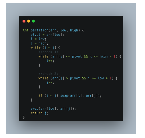
Note: In the function, we have kept the elements equal to the pivot on the left side. If you choose to place them on the right, check 1 will be arr[i] < pivot and check 2 will be arr[j] >= pivot.
C++ Implementation:
What is Linear Search?
Time Complexity:
Worst-case: O(n)
Best-case: O(1)
C++ Implementation:
What is Binary Search?
Time Complexity:
Worst-case: O(logn)
Best-case: O(1)
C++ Implementation:
Last updated